Nonlinear partial differential equations (PDEs) form the mathematical backbone for modeling phenomena across diverse fields such as physics, biology, engineering, and finance. Traditional numerical methods have limitations, particularly for high-dimensional or parameterized problems, due to the "curse of dimensionality" and computational expense. Artificial Intelligence (AI) is currently a valuable tool and has extensive applications in various fields. AI-driven approaches offer a promising alternative by leveraging machine learning techniques to efficiently approximate solutions, especially in high-dimensional or complex problems. This paper first surveys state-of-the-art AI techniques for solving nonlinear PDEs, including Physics-Informed Neural Networks (PINNs), Deep Galerkin Methods (DGM), and Neural Operators. Symbolic computation methods, Hirota bilinear methods, bilinear neural network methods. We explore their theoretical foundations, architectures, advantages, limitations (lacking), and applications. Finally, we discuss the relationship among existing methods and give open challenges and future directions in the field.

1. Introduction

1.1. Background

Nonlinear Partial Differential Equations (PDEs) are fundamental tools in modeling a wide array of complex phenomena across various scientific and engineering disciplines, and often used to describe complex, dynamic systems in fluid mechanics, heat transfer, quantum mechanics, and more. Engineering applications often involve systems where nonlinear PDEs are indispensable. In quantitative finance, nonlinear PDEs are utilized to model various complex financial instruments and markets. These equations model systems where relationships between variables are inherently nonlinear. Their significance stems from their ability to capture intricate behaviors and interactions that linear models cannot adequately represent. Their nonlinearity arises from terms like products of derivatives or nonlinear functions of the solution, leading to phenomena such as shocks, turbulence, and chaos. While traditional methods like finite element methods (FEM), finite difference methods (FDM), and spectral methods, solve PDEs by discretizing the problem into manageable subdomains or points, which are powerful for low-dimensional problems, these methods face scalability issues in high-dimensional scenarios or parameterized problems. As a result, they face challenges such as: 1) High-dimensional Problems: Computational cost scales exponentially with dimension. 2) Complex Boundary Conditions: Irregular domains or dynamic boundaries increase solver complexity. 3) Real-Time Applications: Time-sensitive problems (e.g., weather forecasting) require faster solutions.

Artificial Intelligence (AI), particularly Machine Learning (ML) and Deep Learning (DL), offers a new paradigm for addressing these challenges, and provide flexible and scalable alternatives to traditional methods. AI techniques provide efficient, flexible, and scalable methods to approximate, analyze, and solve nonlinear PDEs, often outperforming traditional numerical methods in specific contexts. So AI-driven methods are very important research directions for solving the nonlinear PDEs, and then we provide the survey for these AI-driven methods of solving the nonlinear PDEs so that readers can understand them in time.

1.2. Motivation

AI methods are attractive due to:

· Mesh-free nature: Mesh-free nature: AI-driven methods like Physics-Informed Neural Networks (PINNs) and Deep Galerkin Methods (DGM) for solving nonlinear PDEs operate without the need for a predefined grid or mesh. This is a significant departure from traditional numerical methods such as finite element methods (FEM), finite difference methods (FDM), and finite volume methods (FVM), which rely on discretizing the computational domain. Instead:

(1) Point-Based Learning: These methods evaluate the solution at scattered points across the domain, which can be sampled randomly or strategically.

(2) Neural Representation: The solution u(x,t) is represented as a continuous function, parameterized by the weights of a neural network (NN). For example: PINNs approximate u(x,t) directly by minimizing the residuals at the sampled points. Points do not need to follow any specific spatial organization (e.g., grid).

· High-dimensional scalability: AI-driven methods can handle problems with a large number of spatial, temporal, or parameter dimensions without significantly increasing computational complexity. Traditional numerical approaches, like finite element methods (FEM) or finite difference methods (FDM), struggle with high-dimensional problems due to the curse of dimensionality, whereas AI methods, particularly neural network-based approaches, excel in this regard.

· Learning capabilities: AI-driven approaches, particularly neural network-based models, combine data-driven and physics-informed strategies. This allows them to handle noisy data or unknown parameters, making them well-suited for solving nonlinear PDEs. These capabilities enable them to generalize across complex domains, learn representations of solutions efficiently, and adapt to variations in physical systems.

1.3. Development Outlines for AI-Driven Nonlinear-PDE Methods

AI-based PDE solvers evolved broadly along two complementary axes:

(1) Physics-constrained, loss-based approximators - networks trained to satisfy PDE residuals and boundary/initial conditions (e.g., PINNs [1], DGM [2], variational PINNs).

(2) Operator-learning and surrogate mapping - networks trained to approximate solution operators mapping inputs (coefficients, initial/boundary data) to solutions (e.g., FNO [3], DeepONet [4]).

Their comparative development timeline (concise) is as follows.

· 1990s–2000s: Early neural PDE solvers (Lagaris et al. [5] and neural ODEs ideas.

· 2017–2019: DGM [2], PINNs [1], PDE-learning (PDE-Net) [6].

· 2019–2021: Operator learning (FNO [3], DeepONet [4]), neural ODEs mainstream [7].

· 2020–2024: Extensions: XPINNs, parareal PINNs, physics-constrained GANs, diffusion models, production frameworks (SimNet, DeepXDE) [8–11].

· 2022–2025: Hybridization, large-scale production, Bayesian PINNs, graph operators, improved theoretical understanding [12–14].

The remainder of this paper is organized as follows: Section 2 provides the survey of AI Techniques for Nonlinear PDEs, Section 3 give out the survey of AI methods for solving exact analytical solutions of nonlinear PDEs, and Section 4 proposes challenges in AI-driven nonlinear PDE Solvers, Section 5 provides conclusion and future directions.

2. AI Techniques for Nonlinear PDEs

Solving nonlinear PDEs is a complex task due to their inherent challenges, such as nonlinearity, high dimensionality, and the sensitivity of solutions to boundary and initial conditions. Artificial Intelligence (AI) offers a diverse range of techniques for tackling these challenges, providing efficient and scalable methods for solving nonlinear PDEs across different domains. Below, we explore the main AI techniques used for solving nonlinear PDEs, along with their methodologies, applications, and strengths.

2.1. Deep Learning Models for Nonlinear PDEs

In this section, we introduce some deep learning methods such as physics-informed neural networks (PINNs), deep galerkin methods (DGM), and neural operators (NeuO) for solving nonlinear partial differential equations (PDEs). The following structural framework diagram (see Figure 1) of three methods, reflecting the differences and connections between different contents (see Table 1).

Figure 1. Structural relationship diagram among PINNs, DGM and NeuO

Table 1. Differences and connections among PINNs, DGM and NeuO

2.1.1. Physics-Informed Neural Networks (PINNs)

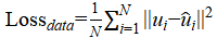
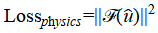
PINNs are introduced and popularized by Raissi et al. [1], and are a specific deep learning approach that integrates the governing PDE into the training process. PINNs leverage the physics of the problem by embedding the PDE residual into the loss function. Raissi et al. [1] directly encoded the differential equation into the loss function, ensuring that the model's predictions adhere to the governing physical laws and suggested the following general physics-informed loss:

where is the residual-weight coefficient weight, often setting to 1.0 (baseline), or dynamically adapted, is the boundary condition weight, and tuned empirically between 1–100 depending on boundary stiffness. is the initial-condition weight, controlling how strongly the model fits the initial state (e.g., u(x,0) = u₀(x)). is to measures how well the solution satisfies the PDE, is to ensure adherence to boundary conditions, is to handle initial conditions, For example, for solving fluid dynamics problems (e.g., 1D viscous Burgers' equation - a simplified 1D form of the Navier–Stokes equation), PINNs used both boundary/initial conditions and the PDE residual in the loss function to enforce physical constraints, where PINN Loss Function (as in Raissi et al. [1] is

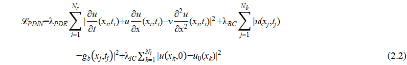
where is the number of residual (collocation) points, is the number of boundary condition points, and is the number of initial condition points. The total training dataset N = N_r + N_b + N_i. Note that PINNs embed the physical laws governing the PDE as soft constraints into the loss function of a neural network (NN). The network predicts the solution u(x,t) by minimizing the residuals of the PDE, boundary conditions, and initial conditions. Its advantages are (1) there is no need for labeled data, and (2) solving forward and inverse problems [1].

However, the PINN method provides only numerical solutions but not exact analytical solutions for PDEs. Thus many researchers further extended PINN frameworks. In the following, we organize these studies into 4 methodological families within the PINN ecosystem. For each family, we will summarize the core idea and point out some limitations, and sketch how they relate to one another. Following [7–9,12,13,15–79], the field has evolved from architectural innovations (see (1): PINN Architecture Extensions) through scalable frameworks (see (2): PINN Software & Scalability) and domain-specific adaptations (see (3): Domain & Problem Extensions ) toward sophisticated training and hybrid methods (see (4): Training Strategies, Inverse Problems & Hybrid Methods ). While each family addresses different facets of PINN research—expressive power, deploy-ability, physics scope, or training robustness—they intersect in their ultimate goal: solving complex PDEs more efficiently, accurately, and reliably by fusing physics knowledge with deep learning.

2.1.1.1. PINN Architecture Extensions (see [8,15–18])

The core idea of this type of methods is to improve the basic PINN by modifying its network architecture or training strategy. Pang et al. [15] extended PINNs to parameter and function inference of integral equations, such as non-local Poisson and non-local turbulence models, and referred to them as non-local PINNs. Non-local physical information neural network nPINNs called parameterized non local pan Laplacian operator. Note that evaluating the parameterized nonlocal Laplacian in [15] required numerical quadrature over a neighborhood, significantly increasing per-iteration cost compared to local PINNs. Meng et al. [8] used a parareal decomposition to tackle long-time PDEs by splitting into coarse and fine subnetworks, and developed the quasi-real physics-informed neural network (PPNN), which decomposes long-time problems into independent short-time problems. But splitting into many short-time PINNs requires coordination between the coarse solver and fine PINNs, introducing synchronization delays in parallel implementations. In 2022, Jagtap et al. [16] proposed a general framework for neural networks with adaptive activation capabilities called Deep Kronecker neural networks. They also introduced local adaptive activation functions for deep and physical information neural networks with slope recovery [17] and adaptive activation functions to accelerate the convergence of deep and physical information neural networks [18]. However, in [16], the Rowdy activation and Kronecker structure add nontrivial operations, potentially offsetting gains from fewer parameters, in [18], dynamically scaling activations may introduce numerical instabilities if the slope grows too large, and stability safeguards are not discussed. Note that [15] and [8,16–18] extended the original PINN framework to overcome its key limitations: slow convergence, inability to handle nonlocal operators, and high computational cost for long-time integration. All in [8,15–18] share the goal of enhancing convergence and expressivity, trading off increased complexity in network design for improved training dynamics and accuracy, but these architectural tweaks often introduce many extra hyper-parameters, complicating training and risking overfitting on limited data.

2.1.1.2. PINN Software & Scalability (see [9,19,20] and [7,24–26])

The core idea of this type of studies is to provide frameworks and computational strategies for efficient, scalable PINN implementation. For example, Lu et al. [19] developed DeepXDE, a deep learning library for solving differential equations based on the Tensorflow version, but suffered from performance overhead, and limited extensibility, and Haghighat et al. [9] developed SciANN, an artificial neural network wrapper based on the Keras/TensorFlow version for deep learning of scientific computing and physical information, but leaded to extra abstraction layers that can impede fine-grained control and efficiency. DeepXDE [19] and SciANN [9] both targeted Python users, lowering barriers but inheriting TensorFlow's complexity. At the same time, Zubov et al. [20] developed an automation software package based on Julia called NeuralPDE to implement physical information neural networks, yet its ecosystem maturity and adoption pose barriers. McClenny et al. [24] developed a scalable multi GPU forward and backward solver, TensorDiffEq, based on TensorFlow 2.x, which provides an intuitive Keras style interface for problem domain definition, model definition, and the use of physics aware deep learning methods for physical information neural networks, yet inherited TensorFlow's version and API constraints. Koryagin et al. [7] developed a Python framework called PyDEns, which uses neural networks to solve differential equations, but it is an early, minimalist Python framework with limited features. Kidger et al. [25] presented Faster ODE Adjointsvia Seminorms, but is mainly theoretical. Rackauckas et al. [26] described a mathematical object (alled Universal Differential Equations (UDEs) ) as a unified framework for connecting ecosystems, but depended on a nascent ecosystem.

These tools above all focused on infrastructure, differing mainly in language (Python vs. Julia), GPU support, and adjoint‐solver integration—they collectively lower the barrier to deploying PINNs at scale. But their Frameworks may abstract away low-level control, making it harder to implement bespoke PDE constraints or hybrid algorithms.

2.1.1.3. Domain & Problem Extensions (see [21–23] and [27–30])

The core idea of this type of studies is to apply PINNs to specialized physics and application domains, or extend them to new equation types. For example, Jin et al. [21] simulated incompressible fluids using physical neural networks, but required careful weight tuning and lacks generalization to other PDE families. In 2021, Hennigh et al. [22] developed a physical machine learning neural network model development framework (called SimNet) to accelerate simulations across various disciplines in science and engineering, but its closed-source components and hardware lock-in limit accessibility. NSFnets [21] and SimNet [22] showcase frameworks optimized for fluid dynamics and multi-physics, respectively. Araz et al. [23] developed a Python package called Elvet, which used machine learning methods to solve differential equations and variational problems, which is a neural network-based solver for differential equations and variation problems, but lacked hardware acceleration. Peng et al. [27] developed a physics based neural network framework – IDRLnet, which provided a structured approach to merge geometric objects, data sources, artificial neural networks, loss metrics, and optimizers, but IDRLnet incurs runtime overhead, and adding novel PINN variants requires digging into internal code rather than simple plugin interfaces. Xiang et al. [28] introduced the adaptive loss balance neural network of incompressible Navier Stokes equation, yet remained case-specific. Note that Elvet [23] and PyDEns [7] offer minimal, standalone solvers, and [14,23,24] and [26] provide code libraries for NN-PDE solving. We could integrate seminorm adjoints [25] and adaptive-loss weights [18] into any of the code stacks [14,23,24,26] to enhance training speed and robustness. The multi-GPU scaling of TensorDiffEq [24] could accelerate large-scale UDEs [26] or lbPINNs [28] experiments. IDRLnet [27], TensorDiffEq [24], SciANN [9], Elvet [23], PyDEns [7] all lower the barrier for PINNs in Python, but differ in extensibility, multi-GPU support, and backend maturity. Wang et al. [29] introduced data-driven rogue waves and discovered parameters in the defocused nonlinear Schrödinger equation using PINN deep learning, but transferring to other PDEs (e.g. reaction-diffusion) remains untested, and the performance with noisy or sparse real measurements is unexplored.. Xu et al. [30] presented a conditional parameterized and discretized perception neural network for grid based modeling of physical systems, but generating weights via trainable functions would add computation overhead compared to static architectures. While all adapt PINNs to new physics, they differ in which layer they intervene—loss function [27,29]), operator form [20]), or entire framework [21–23]). But there are some key limitation - domain specificity can lead to hard-coded constraints, limiting transfer to other physics or PDE families without significant redesign.

2.1.1.4. Training Strategies, Inverse Problems & Hybrid Methods (see [31–42,55–60,68–72,74–79])

The core idea of this type of methods is to tackle training stability, inverse/parameter discovery, and hybrid algorithm designs. They form a spectrum from purely algorithmic fixes (e.g. sampling, failure analysis) to model-based hybrids (e.g. graph, finite-volume), illustrating a progression toward robust, transferable PINN paradigms. But these strategies often require careful hyper-parameter tuning and domain insights to balance multiple loss terms or network modules effectively.

For example, Krishnapriyan et al. [31] introduced the characterization of possible failure modes in physical information neural networks, achieving error reduction of up to 1-2 orders of magnitude, but the analysis for complex multi-physics or chaotic systems is not covered. In 2023, Penwarden et al. [32] studied a unified and scalable framework for causal scanning strategies in physical informed neural networks and its temporal decomposition, but causality and transfer parameters interact in subtle ways, requiring extensive hyper-parameter sweeps.. Yang et al. [33] studied the dynamics of collaborative robots based on human-machine physical interaction and parameter identification based on PINN, and relied on comprehensive sensor data for training, but the performance with fewer sensors or noisier data is unknown. Tian et al. [34] studied data-driven non degenerate bound state solitons in multi-component Bose Einstein condensates based on mixed training PINN, but two-stage “mix-training” introduced extra training passes and prior-info networks, increasing compute cost. Saqlain et al. [35] used PINN to discover the governing equations in discrete systems, and the accuracy depended on suitable initialization of basis terms, but noisy data can degrade symbolic recovery. Liu et al. [36] studied the adaptive transmission of PINN, but note that transfer across very different PDEs can hurt rather than help if mismatch is large. Son et al. [37] studied the physical information neural network (AL-PIN) with enhanced Lagrangian relaxation method, adding inner-loop solves but increasing per-epoch cost. Adaptive activations [17,18], and AL-PINNs [37] tackle training pathologies and multi-objective weighting. One could embed AL-PINN weighting [37] or adaptive activations [17] into IDRLnet [27] or TensorDiffEq [24], then apply causal sweeping [32,33] and transfer strategies [36] for large-scale, multi-GPU PINN solves. Batuwatta Gamage et al. [38] proposed a new physical information neural network method (PINN-MT) to address mass transfer in plant cells during the drying process, but coupling advection–diffusion PINN with cell-geometry constraints may add workflow complexity. Meng et al. [12] proposed a new physics based neural network for reliability analysis of partial differential equations (PINN-FORM), but lacked extension to multi-physics or strongly nonlinear reliability problems beyond the benchmark examples. Liu et al. [39] proposed efficient learning of variational physical information neural network based on region decomposition (cv PINN), and struggled to maintain global solution consistency across subdomains when strong discontinuities or steep gradients are present. Pu et al. [40] proposed a new method called Time Segmented Physical Information Neural Networks (PINNs) to study the complex dynamics of one-dimensional quantum droplets by solving the modified Gross Pitaevskii equation, and tailored to 1D Gross–Pitaevskii dynamics but not validated on higher-dimensional or multi-component quantum systems. Huang et al. [41] proposed a free physics informed neural network using boundary and initial conditions to solve non shallow water free surface problems, but the performance degraded for highly nonlinear free-surface flows due to lack of explicit boundary condition enforcement. Penwarden et al. [42] investigated the application of meta learning methods for physics informed neural networks in parameterized partial differential equations, and focused on forward solves but did not address inverse problems or parameter estimation for unseen PDE families. Guo et al. [43] developed a hydraulic tomography physical information neural network (HT-PINN) for inverting two-dimensional large-scale spatial distribution transmittance, and limited to synthetic 2D cases but lacks assessment on noisy or real-field hydraulic datasets. P. Villarino et al. [44] developed a new strategy using PINNs to handle the boundary conditions of multidimensional nonlinear parabolic partial differential equations, but not evaluate under moving or free-boundary conditions common in financial and physical systems. He et al. [45] combined a multi axis fatigue interface model with a neural network and proposed a physically informed neural network (MFLP-PINN) for life prediction, and relied heavily on available fatigue test data, so limiting its predictive power for novel loading scenarios. Note that both [12] and [45] addressed reliability and fatigue analysis using physics-informed DL, showing practical industrial application potential. Zhang et al. [46] integrated computational fluid dynamics with our customized analysis framework based on multi-attribute point cloud dataset and physical information neural network assisted deep learning module, which may lead to high computational cost and overfitting risk when trained on sparse point-cloud representations of complex vasculature. Yin et al. [47] conducted dynamic analysis of optical pulses based on improved PINN, including soliton solutions, strange waves, and parameter discovery of CQ-NLSE, and this model performance is sensitive to solver hyper-parameters but not tested on experimental optical data. Zhang et al. [48] studied the physics informed neural network with generalized conditional symmetry enhancement and its application in the forward and inverse problems of nonlinear diffusion equations, and imposed symmetry constraints that can lead to training instability and limited applicability to non-symmetric domains. Peng et al. [49] studied the PINN deep learning method for the Liu equation: rogue waves under periodic background, and specialized to periodic backgrounds but not generalized to arbitrary initial or boundary conditions. Wang et al. [50] proposed a method of modifying boundary problems through deep learning algorithms for long-term simulation of NLSE rogue waves or aerator solutions with high numerical errors. Note that long-term stability remains dependent on conventional numerical schemes integrated alongside the PINN, and [46] and [50] integrated traditional CFD/numerical solvers with PINN or DL-enhanced methods for better accuracy and generalization.. Zhu et al. [51] used WL tsPINN to predict the dynamic process and model parameters of vector solitons under high-order coupling effects, but required careful tuning of high-order coupling parameters, hindering out-of-the-box use. Li et al. [52] proposed a hybrid training physics informed neural network and studied the strange waves of the Schrödinger equation based on it, but demonstrated only on noise-free data, with unknown robustness to measurement errors. Pu et al. [53] studied the discovery of vector local waves and parameters in data-driven Manakov systems based on deep learning methods, thus highly tailoring to the Manakov system and lacking benchmarking against other vector PDEs. Zhang et al. [54] applied deep learning methods to study the nonlinear wave solutions of the LPD model describing the evolution of ultra short optical pulses in optical fibers but did not assess on broader optical fiber models. Note that [12,40,47,49–54] focus on applying deep learning (PINNs or variants) to specific nonlinear PDEs including NLSE, CQ-NLSE, Chen–Lee–Liu, and Bose–Einstein models, and all aim to model nonlinear wave propagation or quantum dynamics using physics-aware neural networks, and [43,47,53,54] are concerned with identifying hidden PDE parameters from data, especially in inverse problem setups. After Meng et al. [8] developed a quasi real physics informed neural network (RPINN) , Yuan et al. [55] proposed an auxiliary physical neural network (A-PINN) for the forward and inverse problems of nonlinear integral differential equation, and so got extra auxiliary outputs but still relied on automatic differentiation without addressing the high computational cost of large‐scale integral operators. Gao et al. [56] proposed a unified framework for solving the forward and inverse problems of PDE control, based on a physical graph neural Galerkin network, and so overcomed unstructured meshes but incurred graph‐construction overhead that can limited scalability on very large domains. Yang et al. [13] proposed Bayesian Physical Informed Neural Networks (B-PINNs) for forward and backward PDE problems on noisy data, and provided uncertainty quantification yet was computationally intensive due to HMC or VI sampling in high dimensions. Zhang et al. [57] used the continuous symmetry in physical information neural networks to solve the forward and inverse problems of partial differential equations, and imposed symmetry constraints that improved accuracy but can destabilize training when the true solution only approximately possesses the assumed symmetry. Guo et al. [58] studied a pre training strategy for solving evolutionary equations based on physical information neural networks, and so speeded up convergence via pre‐training but may misguide fine‐tuning if the pre‐trained surrogate poorly matches the target PDE. Guan et al. [59] proposed a high-precision and high-efficiency augmented physical informed neural network (DaPINN), and so achieved higher fidelity by adding auxiliary dimensions but increased network complexity and memory footprint significantly. Luo et al. [60] proposed a hybrid adaptive (HA) sampling method and a feature embedding layer for PINN for dealing with the accuracy and efficiency of PINNs, and balanced accuracy and efficiency with adaptive sampling, yet selecting hyper-parameters for the sampling schedule remains heuristic and problem‐specific. Wang et al. [61] extended a multi-layer PINN and successfully learned data-driven multi soliton solutions, and discovered the coefficients of the fifth order Kaup-Kuperschmidt equation using multi-soliton data, thus learning multi‐soliton dynamics effectively but depending on extensive, high‐resolution training data that may not be available in practice. Tang et al. [62] used a combination of physical informed neural networks and interpolation polynomials to solve nonlinear partial differential equations, and referred to it as Polynomial Interpolation Physical Informed Neural Network (PI-PINN), thus enhancing local accuracy via interpolation but may suffering from Runge's phenomenon on non-uniform grids. Zhong et al. [63] used deep physics information neural networks to study the forward and inverse problems of generalized Gross Pitaevskii equations with complex symmetric potentials, thus handling complex potentials but requiring careful network initialization to converge in the presence of gain–loss terms. Song et al. [64] extended PINNs to learn data-driven stationary and non-stationary solitons of nonlinear Schrödinger equations, and captured stationary and non‐stationary solitons well, yet extension to coupled or higher‐dimensional systems remains untested. Zhou et al. [65] studied the logarithmic nonlinear Schrödinger equation with even and odd time P-symmetric harmonic potentials, and demonstrates both forward/inverse solves but lacks robustness analyses under noisy measurements. Wang et al. [66] applied multi-layer physics informed neural networks for deep learning and successfully studied data-driven peak and periodic peak solutions of some well-known nonlinear dispersion equations with initial boundary conditions, and so discovered peak on dynamics but relied on analytically known solution forms to guide training, limiting black‐box applicability. Note that [40] and [61–66] focused on solitons, rogue waves, and PT‐symmetric systems, demonstrating the versatility of PINN variants in modeling complex wave phenomena, and [13,55,58,65-77] addressed forward/inverse problems, emphasizing physical parameter estimation under noise or incomplete data. Lin et al. [67] designed a two-stage PINN method that adapts the properties of equations by introducing the characteristics of physical systems into neural networks, and so leveraged conservation laws for accuracy but extends training time due to the extra stage. Note that [55-57,59,67] developed new network structures or incorporate symmetry/auxiliary variables to boost representational power, and [56,60,67] exploited graph structures, hybrid sampling, or multi‐stage training to tackle large or stiff PDEs. Wu et al. [68] conducted a comprehensive study on non-adaptive and residual based adaptive sampling of physics informed neural networks, yet did not prescribe a universally optimal strategy, leaving selection to user trial‐and‐error. Note that [13,58,60,68] introduced Bayesian inference, pre‐training, adaptive sampling, or meta‐learning to improve convergence and robustness. Note that [69–71] focused on developing and applying PINN-based methodologies to nonlinear equations and stochastic systems. Qin et al. [69] combined the Weighted Physics Informed Neural Network (WPNN) with the Adaptive Residual Point Distribution (A-WPNN) algorithm to provide an effective deep learning framework for predicting vector soliton solutions and their collisions in coupled nonlinear systems of equations. Note that the A-WPINN method may face scalability issues when applied to high-dimensional systems. Lin et al. [70] proposed two physics informed neural network schemes based on Miura transform and obtained new local wave solutions. Chen et al. [71] proposed a physics informed neural network that calculates the most likely transition path by computing the Euler Lagrange equation. The approach [71] mainly focused on computing the most probable transition paths but may not capture the full spectrum of stochastic dynamics. Hao et al. [72] used graph neural networks to predict the three-dimensional unsteady multiphase flow field in a coal supercritical fluidized bed reactor, which may restrict its applicability to other multiphase flow systems by tailored to a specific reactor setup. Zhang et al. [73] studied the dual phase field model of composite materials with multiple failures, which may lacked the integration with data-driven approaches for enhanced predictive capabilities. Wu et al. [74] proposed an unsupervised data-driven method (Seq SVF) for automatically identifying hidden control equations but may struggle with systems exhibiting high noise levels. Peng et al. [74,80] studied graph convolutional neural networks based on physical information for modeling geometric adaptive steady-state natural convection, limiting its use in transient scenarios. [72] and [75] highlighted the versatility of graph-based approaches in physics-informed modeling. Li et al. [76] studied the motion estimation and system recognition of mooring buoys based on physical information neural networks. Note that the motion estimation method [76] for moored buoys may not account for complex environmental interactions affecting buoy dynamics. Cui et al. [77] developed numerical inverse scattering transformations for the focusing and defocusing Kundu-Eckhaus equations, and its adaptability to other nonlinear systems remains untested. [74] and [77] demonstrated the potential of data-driven techniques in uncovering hidden dynamics. Mei et al. [78] discussed a unified approach combining finite-volume discretization with PINN (FV-PINN) to solve heterogeneous PDEs efficiently, and the FV-PINN framework improves accuracy and efficiency on heterogeneous domains, its reliance on a static finite-volume mesh can limit adaptivity and incur high preprocessing costs for complex geometries. Cohen et al. [79] introduced a physics-informed genetic programming approach (PIGP) to discover underlying PDEs from limited and noisy datasets. The PIGP method excelled at extracting symbolic PDEs from limited data but struggled with computational scalability and robustness when datasets are highly noisy or high-dimensional. Both [78] and [79] addressed the challenge of solving or discovering PDEs under non-ideal conditions—[78] by tightly coupling numerical discretization (finite volumes) with PINNs for heterogeneous domains, and [79] by embedding physics priors into genetic programming for equation discovery—highlighting complementary strategies of mesh-based PINN integration versus symbolic PDE identification in modern AI-driven PDE methodologies.

The significance of PINNs lies in providing a new approach to handle complex physical problems, especially in the absence of large amounts of data. By combining physical equations and neural networks, PINNs can learn the behavior of a system from a small amount of data and be used for prediction and optimization. This method has potential applications in many fields, including fluid mechanics, materials science, astronomy, and more. The advantage of PINNs is that they can improve prediction accuracy by learning physical equations and can be modeled under different boundary conditions and constraints. In addition, PINNs can improve model performance through adaptive learning and can be combined with traditional numerical methods to provide more accurate and efficient solutions. In summary, the significance of PINNs lies in their provision of a new approach for the fields of science and engineering, which can better handle complex physics problems and still provide accurate predictions and optimizations in situations where data is scarce.

2.1.2. Artificial Neural Networks (ANNs)

Artificial Neural Networks (ANNs) are a fundamental tool in AI-based PDE solvers. These networks, particularly deep feed-forward networks, are used to approximate solutions to nonlinear PDEs. Lagaris et al. [5] demonstrated how feed-forward neural networks can be used to solve both ordinary and partial differential equations, highlighting the effectiveness of ANNs in approximating complex solution. Their feed-forward trial‐solution approach [5] mandated hand-crafted incorporation of boundary conditions and did not adaptively focus network capacity on regions with high error, limiting efficiency and scalability to higher‐dimensional domains. Kumar et al. [81] presented GrADE, a graph-based data-driven solver designed to address time-dependent nonlinear PDEs, showcasing its effectiveness through various applications. GrADE's reliance on constructing and traversing large graph representations can introduce significant overhead and memory costs, and its performance has yet to be validated on highly irregular meshes or extremely stiff PDEs.

Both Lagaris et al. [5] and Kumar et al. [81] employed neural networks to approximate PDE solutions, but [5] used a global feed-forward trial function on structured domains, whereas GrADE [81] leveraged a graph neural network on discrete meshes to explicitly capture local connectivity and temporal evolution. For sampling vs. structure: Lagaris et al. [5] accomplished solution approximation by sampling collocation points and embedding boundary conditions analytically, while GrADE [5] encoded the PDE's discrete spatial structure directly into a graph, allowing it to handle unstructured geometries more naturally—albeit at the cost of graph construction overhead. For scalability considerations: The seminal work by Lagaris et al. [5] laid the foundation for mesh-free ANN solvers, whereas GrADE [81] represented a later evolution aiming to scale ANN PDE solvers to complex, time-dependent, and potentially unstructured problems through graph abstractions.

ANNs can approximate highly nonlinear functions due to their layered structure, where each layer transforms the input data nonlinearly.

· Approach: The general approach involves using neural networks to represent the unknown solution u(x,t) of a nonlinear PDE. The network learns to satisfy the PDE by minimizing the residual of the equation during training.

· Example: For a nonlinear heat equation: 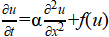, an ANN can be trained to approximate u(x,t) by minimizing the residual: .

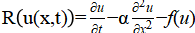2.1.3. Deep Galerkin Method (DGM)

Deep Galerkin Method (DGM) was proposed by Sirignano & Spiliopoulos [2], DGM approximates solution by a deep neural network (NN) and uses Monte-Carlo sampling to evaluate PDE residuals—particularly attractive for high-dimensional PDEs where grids are infeasible. Its algorithmic core is similar to residual minimization as PINNs but often emphasizes stochastic sampling, tailored network architectures (e.g., gating units), and training for backward/forward PDEs (stochastic control, HJB). DGM often targets problems in finance (Black–Scholes, HJB) and high-dimensional control. DGM [2] solves PDEs by approximating the solution u(x,t) with a deep neural network. The network minimizes the variational form of the PDE by sampling points from the domain. Unlike PINNs, DGM focuses on stochastic sampling, making it particularly suited for high-dimensional PDEs [81]. Although DGM can solve up to 200-dimensional free boundary and HJB PDEs without meshes, it relied on sampling from the full domain and lacks error bounds or adaptive sampling strategies to focus learning on regions of interest. Han et al. [82] converted PDEs into BSDE (backward stochastic differential equations) systems and approximate the gradient (“policy”) via deep nets. Their BSDE-based approach [82] mitigated the curse of dimensionality but requires backward stochastic reformulation and can suffer from compounding time-stepping errors in long-horizon or stiff systems. Beck et al. [83] extended the concept of stochastic methods in solving high-dimensional PDEs, discussing DGM as a specific approach. It emphasizes the use of neural networks and stochastic sampling for efficient computation in high-dimensional settings. The merged 2BSDE formulation and temporal discretization in [83] yielded accurate solutions, yet the resulting algorithms remain computationally expensive and sensitive to the choice of network architectures and hyper-parameters.

Note that these methods in [2,82,83] embedded neural networks within stochastic reformulations of PDEs to break the curse of dimensionality: DGM [2] trained on randomly sampled points, akin to a Monte Carlo approach but without explicit variance reduction strategies.Han et al. [81] converted PDEs into BSDE systems and approximate the gradient (“policy”) via deep nets. Beck et al. [83] extended to fully nonlinear PDEs by merging forward–backward SDEs into a single learned recursion.These approaches demonstrated a progression from linear parabolic PDEs (DGM) [2] to semi-linear [82] and finally to fully nonlinear [83] problems, highlighting the power and limitations of stochastic neural solvers.

Thus DGM has itself advantages such as scalability to high-dimensional problems, avoids grid discretization, and efficient sampling strategies for complex domains, and is applied to option pricing in finance (Black-Scholes equation), and reaction-diffusion systems in biology, and so on.

2.1.4. Convolutional Neural Networks (CNNs)

CNNs are particularly useful in solving PDEs that involve image-based data or spatiotemporal dynamics. These networks can capture local features and spatial patterns efficiently. Zhu et al. [84] discussed to use CNNs for modeling high-dimensional, spatiotemporal PDEs while enforcing physical constraints, making them ideal for image-based data. Note that, while leveraging convolutional encoder–decoder networks to enforce PDE constraints without labeled data, the method [84] still requires a structured grid and cannot easily handle complex geometries or unstructured meshes. Long [6] introduced PDE-Net, which used CNNs to learn differential operators and approximate solutions to PDEs, showcasing the suitability of CNNs for spatiotemporal dynamics. By parameterizing convolutional kernels to approximate differential operators, PDE‐Net captures known PDE forms but struggles to identify and generalize to entirely new operator families beyond its assumed discrete stencil patterns. CNNs are widely used in fluid dynamics, image-based simulation problems, and tasks where the solution exhibits local spatial correlations. They can be used to approximate solution fields directly from data, such as predicting velocity or temperature fields. For example: Solving a convection-diffusion equation using CNNs:

Note that both [84] and [78] employed CNNs to approximate spatial derivatives—Zhu et al. [84] embeded these CNNs within a physics‐constrained surrogate model, whereas Long et al. [6] designed learnable convolutional stencils to mimic finite‐difference operators. Both methods [6,84] rely on structured, regular grids: Zhu et al. [84] for the encoder–decoder reshape operations, and PDE‐Net [78] for its convolutional stencils, which limits their applicability to problems on unstructured meshes or complex domains. Zhu et al. [6] focused on surrogate modeling (mapping inputs to solutions under known PDEs) without explicit labels, while PDE‐Net aims at PDE discovery, learning both the solution and the underlying differential operator from data.

2.2. Neural Operators for PDEs

Neural operators (e.g., Fourier Neural Operators (FNOs), DeepONet) learn the solution mapping of PDEs by directly learning the mapping from input functions to output solutions.

2.2.1. Fourier Neural Operators (FNOs)

FNOs are a class of neural networks that operate in the Fourier space, learning the solution operator of PDEs (see Figure 2). They transform the PDE's spatial domain into the frequency domain, applying learned operations in this domain, making them particularly powerful for nonlinear PDEs. FNOs aim to approximate the solution operator of a PDE, G, which maps an input function (e.g., initial condition, boundary condition, or forcing term) to the solution u(x): 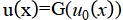. There are key characteristics such as (1) Global Representation: FNOs utilize the Fourier transform to represent the function in the frequency domain, capturing both local and global dependencies. (2) Efficiency: The Fourier transform reduces the complexity of handling high-dimensional inputs and outputs. (3) Flexibility: Applicable to parametric, high-dimensional, and nonlinear PDEs.

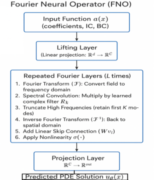
Figure 2. FNO structure - enabling resolution independence and capturing long-range interactions efficiently.

FNOs are particularly well-suited for solving nonlinear PDEs due to their ability to efficiently capture complex interactions in high-dimensional spaces. Examples include: (1) Navier-Stokes Equations: Modeling fluid flow, including turbulence and vortex dynamics. (2) Burgers' Equation: Solving for shock waves in nonlinear advection-diffusion processes. (3) Reaction-Diffusion Systems: Simulating pattern formation in chemical and biological systems. (4) Nonlinear Elasticity: Stress-strain modeling for complex materials. (5) Wave Propagation: Solving nonlinear wave equations in acoustics and electromagnetics.

Li et al. [3] introduced Fourier Neural Operators (FNOs) to demonstrate their ability to efficiently learn solution operators for a variety of parametric PDEs by leveraging the Fourier transform. But FNOs inherently assume periodic or padded domains and can exhibit Gibbs phenomena near discontinuities, limiting their accuracy on non-periodic or highly irregular geometries. Kovachki et al. [14] provided a comprehensive overview of neural operators, including FNOs, and their application to solving nonlinear PDEs in various domains by transforming the problem into the Fourier space, but highlighted that operator‐learning methods often required large training sets of solution snapshots across parameter ranges, making them data-hungry for high-dimensional parameter spaces. Xu et al. [84] considered solving complex spatiotemporal dynamical systems governed by partial differential equations (PDEs) using frequency domain-based discrete learning approaches, such as Fourier neural operators, and proposed a physics- embedded Fourier Neural Network (PeFNN) to enforce conservation laws via additional loss terms, yet the added physics constraints introduce significant computational overhead and hyper-parameter tuning complexity, which can slow training especially in large-scale problems.

Note that Li et al. [3] emphasized spectral efficiency and operator expressivity given ample data and pioneered the data‐driven FNO framework to learn solution operators via spectral convolution, establishing baseline performance on parametric PDEs, and Kovachki et al. [14] highlighted the data-hungry nature of operators and the need for large solution libraries, and Xu et al. [84] seek to inject physics to alleviate data dependence, introducing computational overhead as the trade-off.

2.2.2. DeepONet (Deep Operator Network)

DeepONet is a deep learning framework designed to learn operators between function spaces, enabling it to approximate the solution to a wide class of PDEs. Unlike traditional methods that approximate a solution for a single instance of a PDE, DeepONet learns to approximate the operator itself, enabling rapid solution generation for varying initial conditions, parameters, or source terms. Lu et al. [4] introduced DeepONet, leveraging the universal approximation theorem for operators to solve a wide range of PDEs and learning mappings between infinite-dimensional spaces. Note that DeepONet [4] often required large, paired input–output datasets to train its branch and trunk networks, limiting its practicality when data are expensive or scarce. Wang et al. [85] extended DeepONet by incorporating physics-informed learning to improve the efficiency and accuracy of approximating solutions to parametric PDEs. The method in [85] reduced data needs but depended on judicious tuning of PDE‐residual weights and can struggle with stiff or poorly scaled parametric PDEs. Mouton et al. [86] explored the potential for enhancing a classical deep-learning-based method for solving high-dimensional nonlinear PDEs with suitable quantum subroutines, and constructed a deep-learning architecture based on variational quantum circuits without provable guarantees. The proposed variational quantum‐circuit DeepONet architecture [86] lacked rigorous complexity or error‐reduction guarantees and has yet to demonstrate clear advantage over classical methods. Note that [4] emphasized pure data‐driven operator learning, [85] balanced data with physics priors, and [86] targeted computational acceleration through quantum circuits, illustrating key axes (data, physics, computation) along which neural‐operator research is progressing. All three works in [4,85,86] underscored the need for stronger theoretical analysis to guide practical adoption in real‐world, high‐dimensional PDE tasks.

DeepONet consists of two key networks, one for input functions (e.g., initial conditions) and one for output solutions, to learn the operator between these spaces.

(1) Branch Network:

    Encodes the input function f into a low-dimensional representation.

    Input: Discretized or sampled points of f(x).

    Output: Latent features representing the input function.

(2) Trunk Network:

    Encodes the evaluation points x into another feature space.

    Input: Coordinates where the solution u(x) is to be computed.

    Output: Latent features representing the evaluation points.

Finally, combining outputs from the branch and trunk networks to compute the final solution:

,                                                                          (2.4)

where are the outputs of the branch network and are the outputs of the trunk network.

Still, DeepONet has the following key features.

   Operator Learning: Directly learns a mapping 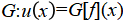, where f is an input function (e.g., boundary conditions, initial conditions, or source terms), and u(x) is the solution.

    Flexibility: Applicable to linear and nonlinear PDEs, and handles parametric PDEs with variable coefficients or source terms.

    Efficiency: Once trained, DeepONet provides real-time solutions for any valid input function fff, bypassing traditional iterative solvers.

     Scalability: Applied to high-dimensional PDEs or systems of PDEs.

The loss function can defined as the difference between the predicted solution and the true solution , typically expressed as:

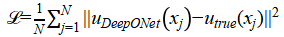                                                          (2.5)

Additional terms may include regularization or physics-informed constraints for PDE consistency.

Applications of DeepONet: Particularly useful for problems where the input function has varying parameters or complex boundary conditions, such as fluid-structure interactions. For example, Navier-Stokes Equations, Burgers' Equation, Reaction- Diffusion Systems, Nonlinear Elasticity, Quantum Mechanics, and so on.

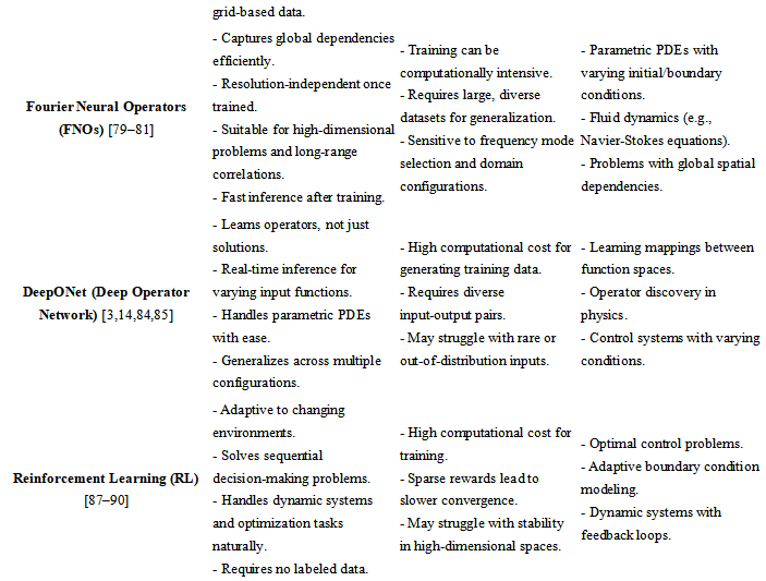
2.3. Reinforcement Learning for PDEs

Reinforcement Learning (RL) is useful for solving optimal control problems involving nonlinear PDEs (see [85]), where the goal is to find a control policy that maximizes or minimizes a specific objective function while satisfying the governing PDEs. Nian et al. [87] provided a review on reinforcement learning for nonlinear PDEs.

· Approach: In this setting, the agent explores possible solutions by interacting with the environment (the PDE), receiving feedback (the objective function), and adjusting its strategy over time. For example, Han et al. [88] demonstrated how RL techniques can solve stochastic control problems, which often involve nonlinear PDEs, by approximating value functions using deep learning methods. Rabault et al. [89] applied deep reinforcement learning to optimal control problems in fluid dynamics, showcasing its capability to handle nonlinear PDEs governing such systems. Bucci et al. [90] explored how RL methods can be adapted for the control of systems described by PDEs, particularly nonlinear dynamics, by framing the control as an optimization problem.

Note that Han et al. [88], Rabault et al. [89], and Bucci & Kutz [90] all pioneered the use of reinforcement learning (RL) for controlling systems governed by nonlinear PDEs. Han & E's early work [88] laid the theoretical groundwork for value‐function approximation in stochastic PDE control, which Rabault et al. [89] extended to fluid‐dynamics benchmarks, and Bucci & Kutz [90] generalized to a broader class of nonlinear PDE control problems. Yet each work of them faces distinct challenges in scaling, robustness, and generality. The deep‐learning approach [88] lacked guarantees on convergence and stability for high‐dimensional PDEs beyond small‐scale benchmarks. The GAN‐based active flow control [89]: excels at drag reduction in 2D vortex shedding but struggles with real‐time adaptation and three‐dimensional turbulent flows due to training‐time complexity and generalization limits. While framing PDE control as an optimization in RL, their method [90] requires extensive sampling of system trajectories, leading to prohibitive data‐efficiency and computational‐cost issues for complex or high‐dimensional domains

· Applications: Used in control problems such as inverse design of systems governed by PDEs, where the goal is to optimize parameters subject to physical constraints.

· Example: Solving a PDE in a control context, such as optimizing the shape of a membrane subject to dynamic forces.

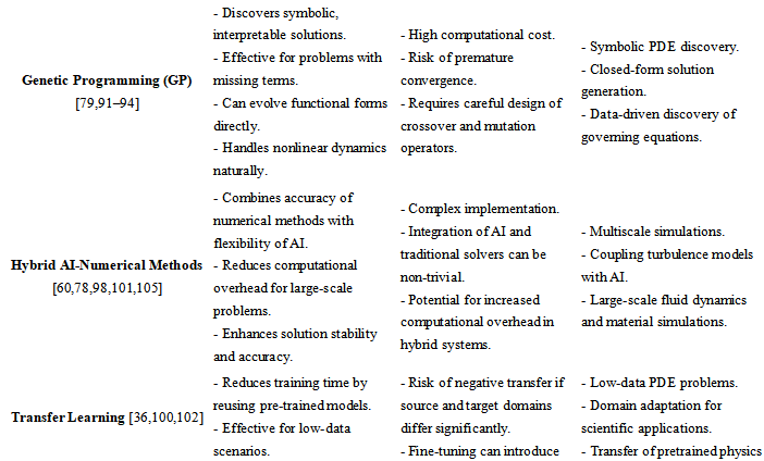
2.4. Evolutionary Algorithms and Genetic Programming

Evolutionary algorithms, such as genetic programming (GP), are used to discover the form of PDEs or approximate solutions through a process of evolution, and optimize mesh structures or adaptive discretization for numerical solvers, and are particularly, well-suited when the problem involves complex landscapes, unknown parameters, or symbolic representation of solutions.

· Approach: GP evolves mathematical expressions or programs over generations, selecting those that best satisfy the PDE's conditions. For example, Jin et al. [91] reviewed multi-objective optimization techniques, including evolutionary approaches, and discusses their applications to discovering and solving PDEs in complex parameter landscapes. While providing a comprehensive survey of Pareto‐based techniques in [91], it did not address the computational challenges of scaling these methods to very high‐dimensional PDE discovery problems. Schmid et al. [92] introduced an approach using genetic programming to discover symbolic representations of governing equations, including PDEs, from data. The genetic programming approach [90] can rediscover known laws but struggles to scale to systems with more than a few variables due to combinatorial explosion. Bongard et al. [93] demonstrated how genetic programming can uncover the structure of nonlinear dynamical systems, which often involve PDEs, through evolutionary exploration, which is effective at uncovering low‐order dynamical structures, but it relied on clean, noise‐free data and degrades rapidly in the presence of measurement error. Deb et al. [94] discussed how genetic algorithms can optimize mesh structures and discretization strategies, providing insights for numerical solvers of PDE and demonstrated mesh and discretization optimization but did not integrate physics constraints directly, limiting its applicability to complex PDE‐driven simulations.

These works in [91–95] applied evolutionary or Pareto‐based strategies to aspects of modeling and solving PDEs. Together, they form a progression from model discovery [92,93] through design optimization [94] to multi‐objective trade‐off handling [78]), illustrating how evolutionary methods can both uncover and refine PDE models across distinct stages of the computational pipeline.

· Applications: Discovering new, unknown forms of nonlinear PDEs or solving highly complex problems where traditional methods may struggle.

2.5. Hybrid AI-Numerical Methods

Hybrid methods combine AI techniques with traditional numerical solvers (e.g., FEM, FDM), leveraging the strengths of both to improve accuracy and efficiency. This approach can improve accuracy, efficiency, and scalability in applications where classical numerical methods face challenges due to complexity, high-dimensionality, or nonlinearity.

· AI techniques such as deep learning are used to extract important features or optimize initial guesses for numerical solvers. And numerical solvers operate on a reduced basis, enhancing efficiency. For data-driven correction, we use numerical methods to solve a coarse version of the PDE, and AI models learn the residual errors and correct the solution iteratively. For example, Raissi et al. [95] demonstrated how AI models, such as neural networks, can be integrated with traditional solvers to approximate fine-scale features by learning residuals. Their “Hidden Fluid Mechanics” framework [95] learned velocity and pressure from flow visualizations but has only been demonstrated on relatively simple 2D flows and may not generalize to complex three-dimensional turbulent regimes. Bar-Sinai et al. [96] illustrated how AI can learn corrections to coarse-grid discretizations for PDEs, blending data-driven methods with traditional numerical solvers, effectively embedding ML into the discretization process. While learning data-driven discretizations on coarse grids improves accuracy for canonical PDEs, the approach in [96] was validated primarily on 1D and 2D toy problems, leaving its extension to large-scale 3D simulations untested. Geneva et al. [97] introduced a framework where AI models learn the discrepancy between numerical solutions and true solutions, iteratively refining the accuracy. Note that the physics-constrained deep auto-regressive networks required sequential time stepping, which can accumulate errors and struggle with long-time stability in highly nonlinear systems. Kashinath et al. [98] explored hybrid approaches where traditional solvers provide a base solution and AI models learn residuals to enhance the accuracy, especially for real-time applications. Their real-time physics-informed ML hybrid exceled for small- to mid-scale PDEs but incurs significant overhead when scaling to large domains or very fine resolutions. Both Raissi et al. [95] and Kashinath et al. [98] train neural networks to learn the discrepancy (residual) between a coarse numerical solution and the true solution, targeting fine-scale features. Rolfo et al. [99] highlighted the integration of machine learning techniques with numerical methods to solve PDEs more efficiently. This perspective piece [99] highlighted ML-numerical integration broadly but lacked concrete algorithmic benchmarks or theoretical analysis to substantiate the claimed efficiency gains.

· Applications: In multi-physics problems or where traditional methods are computationally expensive, AI can help reduce the computational burden or enhance accuracy.

2.6. Transfer Learning for Nonlinear PDEs

Transfer learning enables the reuse of previously learned models for solving similar PDEs with different parameters or domains. By leveraging models trained on a related task, transfer learning reduces the amount of data needed for new problems and accelerates learning. Gupta et al. [100] discussed the application of transfer learning in Physics-Informed Neural Networks (PINNs) to efficiently solve parametric PDEs by reusing pre-trained models. While reusing pre‐trained PINN models accelerates convergence for related parametric PDEs, the work lacks theoretical guarantees or systematic guidelines on how far parameter changes can stretch before negative transfer occurs. Li et al. [3] also demonstrated how Fourier Neural Operators (FNOs) can employ transfer learning to solve PDEs with different parameter distributions, enhancing efficiency and accuracy. FNOs relied on Fourier transforms that exhibit Gibbs oscillations near discontinuities and inherently assume (or require padding for) periodic boundary conditions, which limits their accuracy on problems with strong discontinuities or non‐periodic domains. Ruthotto et al. [101] highlighted transfer learning's potential in neural network models inspired by PDEs, reusing knowledge from related domains to accelerate training for new problems. Although they demonstrate that PDE‐inspired architectures can be fine‐tuned across tasks, they do not empirically evaluate transfer‐learning performance on large‐scale or physically diverse PDE systems. Jin et al. [102] showcases the use of transfer learning in neural networks for solving PDEs across different domains or parameter sets, reducing computational costs significantly, but may suffering from “negative transfer” when the source and target PDE domains differ substantially in physics or geometry. All work in [3] and [100–102] leveraged transfer learning to mitigate the costly retraining of neural PDE solvers when problem parameters change. Li et al. [3] and Gupta & Jacob [100] focused on operator vs. PINN frameworks, respectively, while Ruthotto & Haber [101] bridge both by embedding PDE structure into generic deep nets. Jin et al. [102] then showcase a one‐shot strategy that pushes this concept toward minimal fine‐tuning. These studies illustrate the emerging continuum of transfer‐learning strategies in AI‐driven PDE solvers—from operator learning (FNO) through PINN fine‐tuning to one-shot inference—highlighting both their promise for fast adaptation and the need for deeper theoretical and empirical understanding of transfer limits. None of the works fully characterize transferability bounds, leaving practitioners to empirically tune transfer distances and fine‐tuning schedules.

Steps for applying transfer learning to nonlinear PDEs are as follows:

(1) Source Task Training: Select a nonlinear PDE for which you have sufficient training data or can solve numerically. Train a neural network to approximate the solution using supervised learning or physics- informed approaches (e.g., PINNs). Save the trained model, including learned weights and biases.

(2) Target Task Setup: Identify the target PDE, which is related to the source PDE (e.g., similar boundary conditions, domain geometry, or governing equations with slight parameter changes). Define a new model, often based on the architecture used for the source task.

(3) Weight Initialization: Initialize the target model with the weights from the source model. This provides a good starting point, especially for shared patterns between the source and target PDEs.

(4) Fine-Tuning: Train the target model on the new problem using limited data or domain- specific loss functions. Use a smaller learning rate during fine-tuning to retain useful features from the source model.

Example for solving Navier-Stokes Variants:

(A) Source Task: Train on the incompressible Navier-Stokes equations for a specific Reynolds number.

(B) Target Task: Transfer to a higher Reynolds number or a slightly different forcing term.

(5) Implementation:

(A) Use convolutional neural networks (CNNs) or Fourier neural operators (FNOs).

(B) Pre-train on the source task.

(C) Fine-tune on limited data or residuals from the target PDE.

2.7. Supervised Learning for PDE Solutions

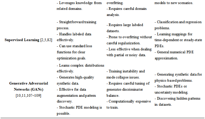
In supervised learning, neural networks are trained using labeled data consisting of PDE input conditions (e.g., boundary values) and corresponding solutions. The model learns the mapping from inputs to solutions directly. For example, Raissi et al. [1] demonstrated how neural networks can map input conditions to solutions using supervised learning techniques. Lusch et al. [103] explored using neural networks to discover embedding of nonlinear dynamics, with applications to solving PDEs through supervised learning on labeled datasets of input conditions and solutions. Note that discovering Koopman embeddings from trajectory data required fully observed state trajectories and then did not directly handle spatially continuous PDE boundary‐value problems. Bhattachary et al. [104] discussed supervised learning techniques for mapping parametric PDE inputs to their solutions, emphasizing neural networks for model reduction. Note that achieving model reduction via supervised mappings may depended on extensive offline sampling of input–output pairs, limiting applicability when sampling is costly or data-scarce. Zhang et al. [105] explored a framework where neural networks learn to solve PDEs without labeled data, using a loss function that incorporates the PDE and boundary conditions. The model generalizes across various domains and boundary conditions, effectively learning the mapping from inputs to solutions. While eliminating labeled data requirements, the CNN encoder–decoder architecture [105] still struggles to generalize in highly irregular geometries outside its training manifold.

Note that these works in [1] and [103–105] frame PDE solving as function-approximation: Raissi et al. [1] and Bhattacharya et al. [104] use supervised neural networks trained on known solution pairs, whereas Lusch et al. [103] leverages auto-encoder architectures to learn latent linear dynamics, and Zhang & Garikipati [105] employs weak-form residuals to remove the need for labels, highlighting a progression from purely data-driven to physics-mediated training paradigms. Both Raissi et al. [1] and Zhang & Garikipati [105] incorporate physics constraints into their loss functions—one via strong enforcement of the PDE residual at collocation points and the other via weak-form integration—while Bhattacharya et al. [104] and Lusch et al. [103] focus on operator learning and model reduction, illustrating complementary strategies for balancing data efficiency and physical fidelity in supervised PDE solvers.

Using supervised learning, its main steps are as follows.

(1) Generate Training Data: We use analytical solutions (if available) or numerical solvers like Finite Difference, Finite Element, or Spectral methods to compute ground truth solutions, and then create input-output pairs (x,t) and u(x,t) over the domain of interest.

(2) Model Design: Input is coordinates x, t; Output: Predicted solution . Then use fully connected neural networks, convolutional neural networks (CNNs), or Fourier neural operators depending on the problem.

(3) Loss Function: The loss function combines data loss and physics loss. Its data loss is to enforce closeness to the ground truth.

                                                               (2.6)

and its physics loss (optional) is to ensure the model satisfies the PDE.

                                                                 (2.7)

Note that total loss is:

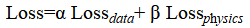                                                        (2.8)

(4) Training: Train the model using a standard optimizer like Adam or SGD, and evaluate performance on validation and test datasets.

(5) Comparison with Physics-Informed Neural Networks (PINNs): Supervised learning requires labeled data (true solutions), while PINNs incorporate the governing equations as part of the loss function, reducing dependency on labeled data. Combining the two methods is also possible for better accuracy.

2.8. Generative Adversarial Networks (GANs)

GANs can be used for solving PDEs by treating the PDE solution process as a generative problem. The generator network produces candidate solutions, and the discriminator network evaluates their validity based on the PDE constraints. For example, Zhu et al. [106] introduced the use of GANs for solving high-dimensional PDEs by generating solutions consistent with physical constraints. While introducing physics-constrained deep learning for high-dimensional surrogate modeling without labeled data, the approach [106] may face challenges in generalizing to complex, nonlinear PDEs due to the reliance on specific physical constraints incorporated into the loss function. Yang et al. [10] explored the use of GANs in inverse problems for PDEs, where the generative model predicts solutions that satisfy the governing equations and boundary conditions. However, the method's performance may degrade when applied to high-dimensional problems or when data is extremely scarce, as the training stability of GANs can be sensitive to such conditions. Xie et al. [107] developed a framework using GANs to approximate PDE solutions while enforcing physical constraints during training. Nonetheless, the approach may struggle with inverse problems where the mapping from observations to solutions is highly non-unique or ill-posed, potentially leading to convergence issues. Sun et al. [108] applied GANs to fluid flow problems governed by PDEs, treating the solution generation as a generative problem with embedded physics constraints. A limitation here is the potential difficulty in capturing complex turbulent flow features accurately, especially in three-dimensional simulations, due to the model's capacity constraints. Lu et al. [11] proposed a Physics-Guided Diffusion Model (PGDM) for downscaling PDE solutions. The model generates high-fidelity approximations from low-fidelity inputs, demonstrating the generative approach to solving PDEs under partial observations. However, the model's reliance on paired low- and high-fidelity data for training may limit its applicability in scenarios where such data is unavailable or expensive to obtain. Mehdi et al. [109] presented a multi-fidelity physics-informed GAN (MF-PIGAN) that utilizes data from various fidelity levels to solve PDEs. The generative model captured complex solution behaviors across different fidelities, enhancing the accuracy of PDE solutions. However, a potential limitation is the complexity involved in balancing and integrating multiple fidelities during training, which may lead to increased computational costs and model tuning challenges.

These studies illustrated the application of GANs in solving PDEs by modeling the solution process as a generative task, effectively capturing complex solution spaces and integrating physical laws into the learning framework. These studies collectively advance the integration of generative models with physical laws to solve PDEs as follows:

(A) Physics Integration: All studies emphasized embedding physical constraints into generative models to ensure that the generated solutions adhere to the underlying PDEs. This integration is crucial for the models to produce physically plausible solutions.

(B) Handling Uncertainty and Data Scarcity: Yang et al. [10] and Taghizadeh et al. [109] addressed uncertainty and data scarcity by incorporating stochastic elements and multi-fidelity data, respectively, into their models. These approaches enhance the models' robustness in real-world scenarios where data may be limited or noisy.

(C) High-Dimensional and Complex Systems: Zhu et al. [106] and Sun et al. [108] focused on high-dimensional surrogate modeling and complex fluid dynamics, demonstrating the applicability of generative models to intricate systems.

(D) Model Efficiency and Scalability: Lu et al. [11] contributed to improving model efficiency by proposing a diffusion model that downscales PDE solutions, highlighting the potential for scalable solutions in computational physics.

In summary, these studies showcase the evolving landscape of using generative models, particularly GANs, in solving PDEs by embedding physical laws into the learning process. While each approach has its limitations, collectively, they pave the way for more robust, efficient, and physically consistent solutions in computational science. However, GANs itself have own key features as follows: (1) The generator learns to produce solutions that minimize the PDE residuals. (2) The discriminator ensures adherence to physical laws by evaluating whether the generated solution satisfies the PDE. Its applications include: turbulence modeling and other high-dimensional stochastic PDEs, and enhancing resolution in numerical simulations. Its advantages include: (1) Handle complex, high-dimensional PDEs. (2) Provides a probabilistic approach, useful for uncertainty quantification. At the same time, there are challenges such as training GANs is notoriously difficult due to mode collapse and instability, and requires careful design of the discriminator to enforce PDE constraints effectively.

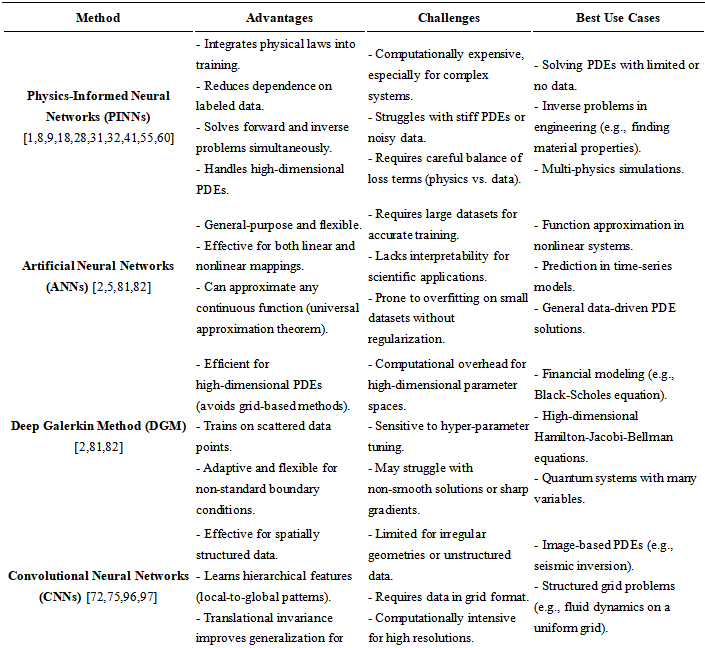
The following is the comprehensive comparison table (see Table 2) for the above techniques across Advantages, Challenges, and Best Use Cases:

Table 2. Comparison among methods

3. AI Methods for Solving Exact Analytical Solutions of Nonlinear PDEs

Nonlinear partial differential equations are mathematical models for many practical problems, but their solutions are often very difficult. As we know, the prerequisite for nonlinear partial differential equations to have exact analytical solutions is that the equation is integrable. The classical neural network methods for solving nonlinear partial differential equations (such as PINNs) can only obtain approximate solutions when used to solve nonlinear partial differential equations in integrable systems.

3.1. Symbolic Computation

Symbolic computation is an important mathematical calculation method that utilizes computers to process and manipulate symbols rather than numerical values. The core idea of symbolic computation is to transform mathematical problems into symbolic expressions and solve them through algebraic operations on these symbols. This method has wide applications in fields such as mathematics, physics, and engineering.

Symbolic computation can also be used for equation solving, differentiation, integration, and other operations, which have important applications in mathematical research and engineering practice. In addition to algebraic operations, symbolic computation can also be applied in fields such as calculus, linear algebra, and discrete mathematics. In calculus, symbolic calculations can be used for limit calculations, derivative calculations, integral calculations, and other operations, helping people better understand the concepts and principles of calculus. Although symbolic computing has a wide range of applications in mathematics and engineering, it also faces some challenges and limitations. Firstly, symbol computation requires a significant amount of computational resources and time, especially when dealing with complex symbol expressions. Secondly, the results of symbolic computation are often in symbolic form and need to be further converted into numerical form in order to be applied to practical problems. In addition, the correctness of symbol calculation also needs to be manually verified to ensure the accuracy of the results. Researchers have developed a large number of symbolic computation methods to solve exact analytical solutions of nonlinear sheet differential equations. For example, Hereman et al. [110] proposed two direct methods for solving solitary wave and soliton solutions and applied them to various nonlinear partial differential equations. The symbolic automations for exact solutions rely on human‐selected ansätze and quickly become intractable for higher‐dimensional or highly nonlinear PDEs.

In addition, there are also F-expansion method [111], Darboux transform method [112], homogeneous balance method [113], Hirota bilinear method [114], Backlund transform [115], Tanh expansion method [116], etc.. In general, symbolic computation is an important mathematical method that solves various mathematical problems by performing algebraic operations on symbols.

Due to the complexity of the classical analysis method based on bilinear transformation, many existing neural network symbolic computation techniques typically require bilinear transformations to linearize nonlinear PDEs before solving them. However, not all integrable nonlinear PDEs have a bilinear form, so analytical methods based on bilinear transformations may not be applicable to all integrable nonlinear PDEs. Hornik showed, in [117], that multilayer perceptron is a universal approximator, it leads that the direct neural network method based on nonlinear transformation will be a universal approach for solving nonlinear partial differential equations (such as (3+1) dimension BLMP equation in integrable systems. Based on the multiple exponential function method, Darvishi et al. [118] studied the multi wave solutions of  (3+1) dimension BLMP equation, and the stair and step solitons via ansatz methods yielded interesting wave forms, but give little insight into stability or parameter‐dependency beyond the chosen ansatz. Liu et al. [119,120] further studies the biperiodic soliton and three wave solutions of such equation. Muhammad et al. [121] studied （2+1） dimension CBS equation. These results  supplement the exact analytical solutions of the (3+1) dimensional BLMP equation and (2+1) dimensional CBS equation in existing literatures (also see [122]).

3.2. Bilinear Neural Network Methods

As we know, the multilayer perceptron model can be seen as a mathematical mapping. Input the independent variable (x; y; z; t), and then map the result f according to the model. In order to obtain exact analytical solutions for nonlinear partial differential equations, Zhang et al. [123] first proposed a bilinear neural network method (BNNM) for solving exact analytical solutions of nonlinear partial differential equations. This BNNM used the mathematical expression of the multilayer perceptron model as the test function and employ a sign based heuristic function method to solve for the exact analytical solution. Note that BNNM has some shortcomings such as its trial and error cost with relatively high. Thus, by providing different neural network model structures and some generalized activation functions, many authors constructed various novel heuristic trial functions to improve the BNNM so that BNNM can be extended and applied to high-dimensional equations, integral differential equations, and other nonlinear partial differential equations. For example, Zhang et al. [124] augments BNNM with residual connections (the Bilinear Residual Network Method), improving convergence on stiffer or higher‐order PDEs. Based on the applications of BNNM, we further explore the following three methodological families as follows.

(1) Applications to Integrable Models (see [124–131])

The core idea of this type of methods is to showcase BNNM's versatility across classic integrable hierarchies - p-gBKP, breaking soliton, Caudrey–Dodd–Gibbon–Kotera–Sawada, and Jimbo–Miwa equations—by extracting bright, dark, lump, and rogue‐wave solutions. For example, for p-gBKP equation, [125–129] catalog interference waves, bright–dark soliton interactions, and dimensional reductions via BNNM. For breaking soliton & Caudrey–Dodd–Gibbon–Kotera–Sawada (CDGKS), [124,126,127,130], introduce novel trial functions to capture rogue waves and generalized lump solutions in 2+1D settings. For Jimbo–Miwa (3+1D), [128] and [131]  extend BNNM to higher dimensions, extracting high‐order rogue‐wave profiles. The p-gBKP cluster [125–129] progresses from basic bright–dark solitons to multi‐soliton and periodic solutions. The breaking‐soliton branch [124,126,127,130] shares ansätze but diverges in PDE form, revealing BNNM's adaptability across sibling hierarchies.The key Limitations of these methods are to craft bespoke neural architectures and bilinearizations, impeding a unified solution framework, and to remain within integrable or near‐integrable regimes for all targets so that nonintegrable PDEs are unaddressed.

(2) Periodic, Breather & Interaction Phenomena (see [132-139])

The core Idea of this type of methods is to employ BNNM to unearth periodic, breather, and interaction dynamics—including fission, rogue–breather hybrids, and mixed soliton–breather patterns—on constant and variable backgrounds. BLMP Equations in [132,133] systematically derived three periodic solution families and lump–stripe interactions for the Boiti–Leon–Manna–Pempinelli model, and shared a core bilinear form and differences arise from the choice of periodic vs. lump ansatz inputs. High‐Dimensional Evolution Models in [134–139] captured breather, rogue, and multiwave interactions in KP, Sharma–Tasso–Olver, and generalized soliton equations, including fission and annihilation phenomena. They extended the same BNNM scaffold to ever‐richer interaction scenaria, demonstrating methodological continuity. There are some key limitations such as complex backgrounds - training becomes more delicate as solution landscapes gain modulation or variable‐coefficient complexity; black‐box nets can obscure underlying physics, and ansatz transparency - the learned trial functions for periodicity are not easily interpretable in classical function‐expansion terms.

(3) Extensions to Fractional, Non-Integrable & Stochastic PDEs (see [129,134,140,141])

The core idea of this types of methods is to test BNNM's frontiers by tackling fractional PDEs, Fokker–Planck equations, and newly discovered integrable systems, crossing into stochastic and non-integer domains. Fractional BNNM in [134] integrated Caputo derivatives into the bilinear‐neural framework, enabling exact‐form solutions of fractional evolution equations. Neural Fokker–Planck Solvers in [140] and [141] demonstrated that BNNM‐style networks can recover analytical propagators and steady states of Fokker–Planck dynamics. And new Integrable Equations in [129] broadened the repertoire of PDEs to which BNNM can potentially apply, laying groundwork for future expansions. Note that these works in [129,134,140,141] collectively test BNNM's flexibility—from classical solitons to nonlocal and stochastic PDEs—indicating a path toward a universal analytical neural solver. At the same, there are some key limitations such as fractional and stochastic integrals demand careful quadrature and stability analysis, challenging the “exact” promise, and neural Fokker–Planck solvers may struggle with capturing heavy tails or metastability exactly. In order to overcome the shortcomings of BNNM, experts construct various trial functions. Zhang and Li et al. [124] proposed a bilinear residual network method (BRNM) to improve the corresponding trial function. As we know, the activation function of the last layer in fully connected neural network models cannot interact with the neurons inside the network. However, through residual networks, shallow neurons can be transmitted to the inside of the neural network model, achieving internal interactions within the network. By utilizing this characteristic, the trial function constructed using residual network models can provide more interactive results, thereby increasing the probability of obtaining accurate explicit solutions. This BRNM belongs to the intelligent symbolic computing technology for solving exact analytical solutions of nonlinear partial differential equations, and has the following three advantages: (1) It has higher accuracy than classical neural network methods for solving PDEs, and can obtain 100% accurate analytical solutions; (2) Unify a large number of classic probing letters Numerical method; (3) This lays the foundation and provides a path for the universal solution of symbolic computation for nonlinear partial differential equations in integrable systems. In addition, based on the bilinear neural network method, this method utilizes a residual network model to improve the corresponding trial function.

Figure 3. Comparison between BNNM and PINNS algorithms

Figure 3 shows the comparison between BNNM and PINNS algorithms, from which it can be seen that both PINNs algorithm and BNNM construct the solution u of the original equation through neural networks. The difference is that PINNs algorithm transforms solving partial differential equations into optimization problems, while BNNM transforms solving partial differential equations into solving systems of equations. We further see that the neural–tau functions in [112–121] acted as adaptive ansatzes, unifying classical functional‐expansion methods under a trainable, data‐driven umbrella. [123] established BNNM's architecture; [124–130,142] and [131-133,135-139,143,] instantiated it on integrable hierarchies and interaction phenomena, and remained integrated with Hirota's theory; [129] and [140,141,144] pushed its boundaries into fractional and stochastic realms, and leaded BNNM toward non-integrable and non-integer PDEs.

4. Challenges in AI-Driven Nonlinear PDE Solvers

AI-driven methods for solving nonlinear partial differential equations (PDEs) have demonstrated significant promise, but they also face several challenges. These hurdles range from computational complexity to limitations in generalization and scalability. Addressing these challenges is essential for the widespread adoption of AI-based PDE solvers in real-world applications. Traditional numerical methods may face many issues such as convergence, stability, and computational complexity when dealing with nonlinear equations. In addition, there is currently no universal method for traditional analytical solutions. The method based on neural network symbolic computation (symbolic reasoning) provides a new approach to better solve the challenges of nonlinear partial differential equations, which can make deep learning more interpretable and explainable, providing new ideas for the application of deep learning in scientific research (such as the solving of nonlinear partial differential equations) and engineering applications.

4.1. Challenges

(1) Computational Complexity

(A) Training Time: Training deep neural networks for complex nonlinear PDEs can be computationally expensive, especially for large domains or high-dimensional problems.

Example: PINNs require solving the PDE over many points iteratively, which can result in slow convergence for stiff PDEs like the Navier-Stokes equations.

(B) Memory Requirements: Handling high-dimensional PDEs or large neural networks requires significant memory, especially for methods relying on automatic differentiation.

(C) Resource-Intensive Optimization: Optimizing neural networks involves large-scale matrix operations and gradients computation, which can be resource-intensive for multi-physics PDEs or fine-grained solutions.

(2) Generalization and Extrapolation

(A) Limited Generalization to Unseen Domains: AI models may generalize well within the training domain but struggle to extrapolate to new or unseen domains.

Example: A PINN trained on one geometry may require retraining to adapt to different boundary conditions or domain shapes.

(B) Overfitting to Sampling Points: Poor sampling strategies can lead to overfitting to specific sampled regions, resulting in inaccuracies elsewhere in the domain.

(3) Data Dependency

(A) Data-Driven Models: Methods that rely heavily on data (e.g., supervised neural networks) are only as good as the quality and quantity of available data.

Example: Sparse or noisy experimental data can lead to poorly learned solutions.

(B) Balancing Data and Physics: Striking a balance between data-driven and physics-informed components is challenging, especially for hybrid approaches.

(4) Handling Stiffness and Nonlinearity

(A) Stiff PDEs: characterized by widely varying scales or rapid changes, pose significant training difficulties. Neural networks may struggle to learn stable solutions in such cases.

Example: The Burgers' equation with a small viscosity parameter results in sharp gradients that are hard to capture.

(B) Strong Nonlinearities: Highly nonlinear PDEs can lead to unstable training and convergence issues. Loss landscapes for such problems may contain many local minima, making optimization challenging.

(5) Loss Function Design and Balancing

(A) Multi-Term Loss Functions: Loss functions in AI-driven solvers often involve multiple terms: residuals, boundary conditions, initial conditions, etc. Balancing these terms during training is non-trivial.

Example: Weighting boundary condition losses too heavily may compromise accuracy in the interior of the domain.

(B) Vanishing Gradients: Loss terms for certain conditions may diminish during training, causing imbalanced optimization and affecting solution accuracy.

(6) Sampling Strategies

(A) Uniform vs Adaptive Sampling: Uniform sampling may miss critical regions like high-gradient areas, while adaptive sampling increases computational complexity.

Example: In turbulent flow simulations, under-sampling near vortices can lead to inaccurate solutions.

(B) High-Dimensional Sampling: Sampling effectively in high-dimensional spaces is challenging, as the number of required samples grows exponentially with dimensionality.

(7) Scalability to Real-World Problems

(A) Large-Scale Domains: Scaling AI solvers to large domains or complex geometries often requires significant computational resources.

Example: Climate models with large domains and multi-scale interactions are computationally demanding.

(B) Multi-Scale and Multi-Physics Problems: Solving PDEs with phenomena occurring across different scales or involving coupled physics (e.g., fluid-structure interactions) remains a challenge.

(8) Numerical Stability and Convergence

(A) Training Instability: Training neural networks for PDE solutions can suffer from instability due to exploding or vanishing gradients.

Example: Oscillatory solutions in wave equations are prone to unstable training dynamics.

(B) Convergence Guarantees: Unlike traditional numerical solvers with well-established convergence theories, AI-driven methods lack robust theoretical guarantees of convergence and accuracy.

(9) Interpretability

(A) Black-Box Nature: Neural networks are often criticized for being black boxes, offering little insight into how solutions are generated or what features are being captured.

Example: Understanding how a neural network captures boundary layer phenomena in fluid dynamics is non-trivial.

(B) Diagnostic Tools: AI-driven solvers lack reliable tools for diagnosing and interpreting errors in learned solutions.

(10) Integration with Existing Frameworks

(A) Hybrid Methods: Integrating AI methods with traditional solvers (e.g., FEM, FDM) introduces compatibility issues.

Example: Transitioning between AI-generated and FEM-based solutions for different regions of a domain can lead to inconsistencies.

(B) Legacy Systems: Many industries rely on well-established numerical frameworks. Adopting AI methods requires significant infrastructure changes.

(11) Lack of Standardization: There is no standardized framework for AI-based PDE solvers, leading to variations in implementations and results. Thus developing unified benchmarks and evaluation metrics is essential for consistency.

(12) Ethical and Practical Concerns

(A) Reliability in Safety-Critical Applications: AI methods must demonstrate high reliability for applications like medical simulations, aerospace engineering, or nuclear reactor modeling.

(B) Energy and Resource Usage: Training large-scale models for PDE solutions can have a significant environmental footprint due to energy consumption.

4.2. Strategies to Address Challenges

(1) Enhanced Sampling: Use adaptive sampling to focus on critical regions, reducing computational cost while maintaining accuracy.

(2) Advanced Optimization Techniques: Leverage advanced optimization methods like second-order optimizers, adaptive learning rates, or reinforcement learning for better training stability.

(3) Hybrid Approaches: Combine AI methods with traditional numerical solvers to exploit the strengths of both.

(4) Explainable AI: Develop interpretable AI models that provide insights into learned solutions and decision-making processes.

(5) Transfer Learning and Pre-training: Use transfer learning to leverage pre-trained models, reducing training time for similar PDEs or domains.

(6) Parallelization and High-Performance Computing: Employ GPUs, TPUs, or distributed computing frameworks to accelerate training and inference.

5. Conclusion and Future Directions

AI-driven methods for solving nonlinear PDEs represent a transformative shift in computational science. By combining physics-informed learning with data-driven approaches, these methods offer solutions to problems previously intractable with traditional solvers.

A significant emerging trend is the application of Transformer architectures, which have revolutionized natural language processing, to the domain of PDEs. The self-attention mechanism inherent in Transformers is exceptionally well-suited for capturing long-range, multi-scale dependencies in spatiotemporal data, a key challenge in simulating phenomena like turbulence or wave propagation over large domains. Future research could explore replacing or augmenting the core networks in frameworks like Fourier Neural Operators (FNOs) or DeepONet with Transformer-based encoders. This integration could lead to more effective solution operators for PDEs with highly non-local effects. Furthermore, Transformer-based models show great promise for learning directly from sequences of simulation data, potentially enabling predictive models that understand temporal dynamics more profoundly than current recurrent or convolutional approaches. The primary challenges will be mitigating the substantial computational cost of self-attention and developing efficient spatial-temporal tokenization strategies for continuous fields.

However, challenges like interpretability, stability, and scalability need to be addressed for broader adoption.

(1) Hybrid Approaches: Combining AI with traditional numerical methods for enhanced accuracy and stability.

(2) Transfer Learning: Using pretrained models for related PDEs to reduce computational cost.

(3) Explainable AI: Developing interpretable architectures to improve trust in AI solvers.

(4) Real-Time Applications: Optimizing AI solvers for time-critical applications like weather forecasting.

Author Contributions: Conceptualization, M.L. and R.Z.; methodology, M.L.; validation, M.L., J.G. and R.Z.; formal analysis, J.G.; investigation, M.L.; resources, J.G.; writing—original draft preparation, J.G.; writing—review and editing, M.L.; visualization, J.G.; supervision, R.Z.; project administration, R.Z.; funding acquisition, M.L. All authors have read and agreed to the published version of the manuscript.

Funding: This paper is supported by the National Nature Science Foundation of China under grant number: 62466025.

Ethical Approval: Not applicable.

Informed Consent Statement: Not applicable.

Data Availability Statement: Not applicable.

Acknowledgments: Not applicable.

Conflicts of Interest: The authors declare no conflicts of interest.